PROMISCES: Norman Lists
Michael Rustler
2022-09-06 05:33:36
Source:vignettes/promisces_norman-lists.Rmd
promisces_norman-lists.RmdInstall R Package
# Enable this universe
options(repos = c(
  kwbr = 'https://kwb-r.r-universe.dev',
  CRAN = 'https://cloud.r-project.org'))

# Install R package
install.packages('wasserportal')
Get Norman Lists
library(wasserportal)

download_file <- function(url,
                            tdir = tempdir()
) {
filename <- basename(url)
t_path <- file.path(tdir, filename)
download.file(url, dest= t_path, mode="wb")
t_path
}

### Download S0 | SUSDAT | Merged NORMAN Suspect List: SusDat
### Version: NORMAN-SLE-S0.0.4.1 (2021-01-18)
### DOI: 10.5281/zenodo.5873975

norman_s0_path  <- download_file("https://zenodo.org/record/5873975/files/susdat_2022-01-18-104316.csv")
norman_s0 <- readr::read_csv(norman_s0_path)
#> Warning: One or more parsing issues, see `problems()` for details
#> Rows: 109631 Columns: 68
#> ── Column specification ────────────────────────────────────────────────────────
#> Delimiter: ","
#> chr (41): Norman_SusDat_ID, Name, Name_Dashboard, Name_ChemSpider, Name_IUPA...
#> dbl (27): PubChem_CID, Monoiso_Mass, M+H+, M-H-, Pred_RTI_Positive_ESI, Pred...
#>
#> ℹ Use `spec()` to retrieve the full column specification for this data.
#> ℹ Specify the column types or set `show_col_types = FALSE` to quiet this message.

### Download S36 | UBAPMT | Potential Persistent, Mobile and Toxic (PMT) substances
### Version: NORMAN-SLE-S36.0.2.1 (2020-12-15)
### DOI: "10.5281/zenodo.4323239"

norman_s36_ubapmt_path  <- download_file("https://zenodo.org/record/4323239/files/S36_UBAPMT_Dec2020.csv")
norman_s36_ubapmt <- readr::read_csv(norman_s36_ubapmt_path)
#> Rows: 258 Columns: 35
#> ── Column specification ────────────────────────────────────────────────────────
#> Delimiter: ","
#> chr (33): CAS_Number, Name, List, ProtectedCAS, REACH_Emission_Likelihood, P...
#> dbl  (2): Largest_Fragment_mass, PubChemCID_largestFragment
#>
#> ℹ Use `spec()` to retrieve the full column specification for this data.
#> ℹ Specify the column types or set `show_col_types = FALSE` to quiet this message.


### Download S90 | ZEROPMBOX1 | ZeroPM Box 1 Substances
### Version: Version NORMAN-SLE-S90.0.1.0 (2021-01-15)
### DOI: 10.5281/zenodo.5854252

norman_s90_zeropm_path  <- download_file("https://zenodo.org/record/5854252/files/ZeroPM_Box1.csv")
norman_s90_zeropm <- readr::read_csv(norman_s90_zeropm_path)
#> New names:
#> Rows: 38 Columns: 13
#> ── Column specification
#> ──────────────────────────────────────────────────────── Delimiter: "," chr
#> (11): CAS, Name, DTXSID, InChIKey, SMILES, InChI, MolecularFormula, IUPA... dbl
#> (2): PubChem_CID, MonoisotopicMass
#> ℹ Use `spec()` to retrieve the full column specification for this data. ℹ
#> Specify the column types or set `show_col_types = FALSE` to quiet this message.
#> • `Synonym` -> `Synonym...11`
#> • `Synonym` -> `Synonym...12`
#> • `Synonym` -> `Synonym...13`


cas_wasserportal <- wasserportal::readPackageFile(file = "cas_wasserportal.csv",
                                                  encoding = "UTF-8")
cas_reach <- wasserportal::readPackageFile(file = "cas_reach.csv")

ubapmt_publication <- cas_reach %>%
  dplyr::filter(.data$cas_number %in% unique(cas_wasserportal$cas_number))


ubapmt_zenodo <- norman_s36_ubapmt %>%
  dplyr::filter(.data$CAS_Number %in% unique(cas_wasserportal$cas_number)) %>%
  dplyr::rename(cas_number = .data$CAS_Number)

missing_on_zenodo <- cas_reach %>%
  dplyr::mutate(zenodo = dplyr::if_else(.data$cas_number %in% unique(ubapmt_zenodo$cas_number),
                                        "yes",
                                        NA_character_),
                publication = dplyr::if_else(.data$cas_number %in% unique(ubapmt_publication$cas_number),
                                        "yes",
                                        NA_character_)) %>%
  dplyr::filter(publication == "yes" | zenodo == "yes") %>%
  dplyr::relocate(tidyselect::all_of(c("publication", "zenodo")), .before = .data$emission_likelihood)


DT::datatable(missing_on_zenodo, filter = "top", rownames = FALSE)Get GW Quality from Wasserportal
# Load R package

### For details see:
### https://kwb-r.github.io/wasserportal/articles/groundwater.html
### JSON files (see below) are build every day automatically at 5a.m. with
### continious integration, for build status, see here:
### https://github.com/KWB-R/wasserportal/actions/workflows/pkgdown.yaml

### GW quality (all available parameters!)
gwq_master <- jsonlite::fromJSON("https://kwb-r.github.io/wasserportal/stations_gwq_master.json")
gwq_data <- jsonlite::fromJSON("https://kwb-r.github.io/wasserportal/stations_gwq_data.json") %>%
  dplyr::filter(.data$Parameter %in% cas_wasserportal$Parameter) %>%
  dplyr::inner_join(cas_wasserportal, by = "Parameter") %>%
  dplyr::inner_join(norman_s0_in_wasserportal, by = "cas_number") %>%
  dplyr::filter(.data$logKow_EPISuite <= 4.5,
                !is.na(.data$`LC50_48_hr_ug/L`)) %>%
  dplyr::mutate(Messstellennummer = as.character(Messstellennummer),
## CensorCode: either "below" (less than) for concentration below detection limit
## (value is detection limit) or "nc" (not censored) for concentration above
## detection limit
                CensorCode = dplyr::case_when(Messwert <= 0 ~ "lt",
                                              TRUE ~ "nc"),
                Messwert = dplyr::case_when(Messwert < 0 ~ abs(Messwert),
### Only two decimal numbers are exported by Wasserportal, but some sustances
### have lower detection limit, e.g. 0.002 which results in -0.00 export, thus
### the dummy detection limit 0.00999 was introduced (until fixed by Senate:
### Christoph will sent a email to Matthias Schröder)
                                            Messwert == 0 ~ 0.009999,
                                            TRUE ~ Messwert)) %>%
  dplyr::left_join(gwq_master, by = c("Messstellennummer" = "Nummer"))

gwq_subs <- gwq_data %>%
  dplyr::count(.data$cas_number, .data$CensorCode) %>%
  tidyr::pivot_wider(names_from = CensorCode, values_from = n) %>%
  dplyr::mutate(lt = ifelse(is.na(lt), 0, lt),
                nc = ifelse(is.na(nc), 0, nc),
                n_total = lt + nc,
                percent_nc = 100*nc/n_total) %>%
  dplyr::rename(n_lt = lt,
                n_nc = nc) %>%
  dplyr::left_join(norman_s0_in_wasserportal) %>%
  dplyr::rename(name_norman = .data$Name_Dashboard)
#> Joining, by = "cas_number"

 readr::write_csv(gwq_subs, "gwq_subs.csv")
DT::datatable(gwq_subs, filter = "top", rownames = FALSE)Norman Substances in Wasserportal
Filter criteria: - log Kow (column logKow_EPISuite <= 4.5) - toxicity value (column LC50_48_hr_ug/ not NA)
gwq_subs_plot <- samples_by_para_and_station_n %>%
  dplyr::filter(.data$percent_samples_abovedetection > 0) %>%
  dplyr::left_join(norman_s0_in_wasserportal) %>%
  dplyr::arrange(.data$`LC50_48_hr_ug/L`) %>%
  dplyr::mutate(label = sprintf("%s (%s, LC50_48_hr_ug/L: %.1f, logKow_EPISuite: %.1f : ",
                                .data$name_norman,
                                .data$cas_number,
                                .data$`LC50_48_hr_ug/L`,
                                .data$logKow_EPISuite
                                ))
#> Joining, by = "cas_number"

gwq_subs_plot$label <- as.factor(gwq_subs_plot$label)
g1 <- gwq_subs_plot %>%
  ggplot2::ggplot(ggplot2::aes(x = .data$percent_samples_abovedetection,
                               y = forcats::fct_reorder(.data$label, .data$percent_samples_abovedetection, .desc = TRUE),
                               label = sprintf("%2.2f %% (n_samples = %d, n_stations = %d)", .data$percent_samples_abovedetection,.data$n_total, .data$n_stations_sampled),
                               fill = .data$logKow_EPISuite)) +
  #ggplot2::scale_fill_brewer(palette="RdYlGn") +
  ggplot2::scale_y_discrete(limits = rev) +
  ggplot2::geom_bar(stat = "identity") +
  ggplot2::geom_text(size = 1.8, hjust = -0.01) +
  ggplot2::xlim(c(0,120)) +
  ggplot2::theme_bw() +
  ggplot2::theme(legend.position = "top") +
  ggplot2::labs(#subtitle = sprintf("%d / %d substances (>= 1 value above detection limit)",
                #                sum(gwq_subs_plot$n_abovedetection > 0),
                #                   nrow(gwq_subs_plot)),
                y = "",
                x = "Percent of Samples above Detection Limit (%)")

g1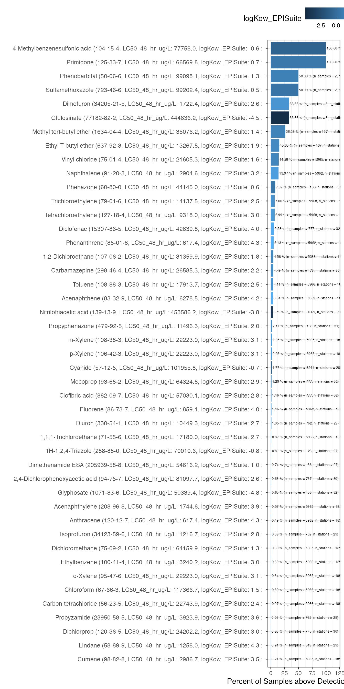
ggplot2::ggsave(filename = "wasserportal_norman-s0-substances_only-above-detection-limit.jpeg",
                  plot = g1,
                  width = 40,
                  height = 20,
                  units = "cm")