How to work with the kwb.qmra package in R(Studio) is described in the following chapters
Once the R package is installed it can be loaded with the following command in R(Studio):
1 Input data
1.1 Location of ‘dummy’ configuration
The folder with the csv configuration files for a hypothetical use case is located here:
#### DEFINE DIRECTORY ################
confDir <- system.file("extdata/configs/dummy", package = "kwb.qmra")
confDir
## [1] "/Users/runner/work/_temp/Library/kwb.qmra/extdata/configs/dummy"The following screenshot shows the required configuration files located in confDir (here: /Users/runner/work/_temp/Library/kwb.qmra/extdata/configs/dummy):
Screenshot of required configuration files
1.2 Import configuration into R
All csv files with the input data for the hypothetical u dummy (as shown above) are imported into R with the following function:
#### LOAD ############################
config <- config_read(confDir)
2 Check input data
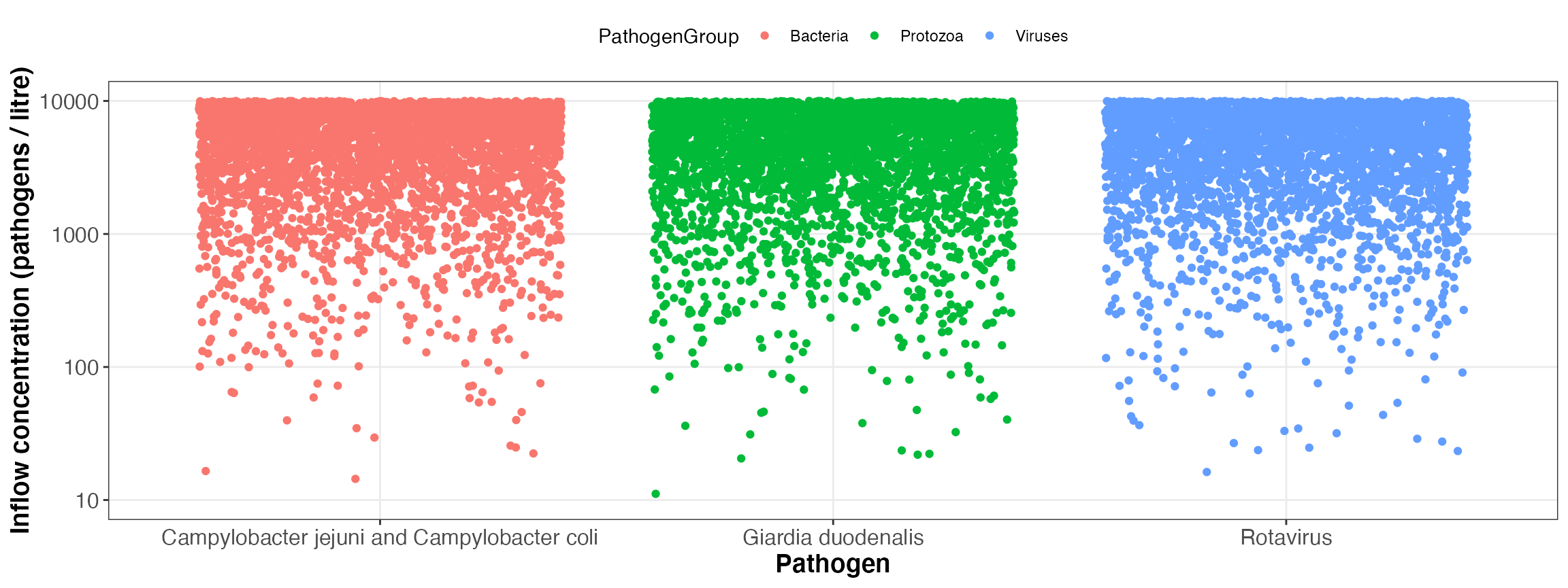
The QMRA will be performed - in case the user does not modify them in R - based on the imported input data, which are defined in the configuration folder.
In case of the dummy configuration, a Monte carlo simulation (n = 10) for 365 exposure events per year for three pathogens and the following input parameters will be performed:
| PathogenID | PathogenName | PathogenGroup |
|---|---|---|
| 3 | Campylobacter jejuni and Campylobacter coli | Bacteria |
| 32 | Rotavirus | Viruses |
| 36 | Giardia duodenalis | Protozoa |
| PathogenID | PathogenName | PathogenGroup | type | min | max |
|---|---|---|---|---|---|
| 3 | Campylobacter jejuni and Campylobacter coli | Bacteria | uniform | 10 | 10000 |
| 32 | Rotavirus | Viruses | uniform | 10 | 10000 |
| 36 | Giardia duodenalis | Protozoa | uniform | 10 | 10000 |
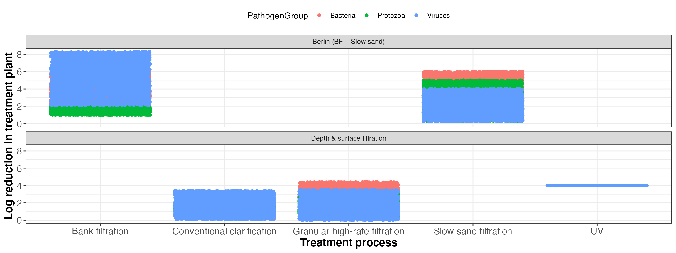
| TreatmentSchemeID | TreatmentSchemeName | TreatmentID | TreatmentName |
|---|---|---|---|
| 1 | Berlin (BF + Slow sand) | 8 | Slow sand filtration |
| 1 | Berlin (BF + Slow sand) | 9 | Bank filtration |
| 2 | Depth & surface filtration | 1 | Conventional clarification |
| 2 | Depth & surface filtration | 5 | Granular high-rate filtration |
| 2 | Depth & surface filtration | 15 | UV |
| TreatmentID | TreatmentName | TreatmentGroup | PathogenGroup | type | min | max |
|---|---|---|---|---|---|---|
| 1 | Conventional clarification | Coagulation, flocculation and sedimentation | Bacteria | uniform | 0.20 | 2.0 |
| 1 | Conventional clarification | Coagulation, flocculation and sedimentation | Protozoa | uniform | 1.00 | 2.0 |
| 1 | Conventional clarification | Coagulation, flocculation and sedimentation | Viruses | uniform | 0.10 | 3.4 |
| 5 | Granular high-rate filtration | Filtration | Bacteria | uniform | 0.20 | 4.4 |
| 5 | Granular high-rate filtration | Filtration | Protozoa | uniform | 0.40 | 3.3 |
| 5 | Granular high-rate filtration | Filtration | Viruses | uniform | 0.00 | 3.5 |
| 8 | Slow sand filtration | Filtration | Bacteria | uniform | 2.00 | 6.0 |
| 8 | Slow sand filtration | Filtration | Protozoa | uniform | 0.30 | 5.0 |
| 8 | Slow sand filtration | Filtration | Viruses | uniform | 0.25 | 4.0 |
| 9 | Bank filtration | Pretreatment | Bacteria | uniform | 2.00 | 6.0 |
| 9 | Bank filtration | Pretreatment | Protozoa | uniform | 1.00 | 2.0 |
| 9 | Bank filtration | Pretreatment | Viruses | uniform | 2.10 | 8.3 |
| 15 | UV | Primary disinfection | Bacteria | uniform | 4.00 | 4.0 |
| 15 | UV | Primary disinfection | Protozoa | uniform | 4.00 | 4.0 |
| 15 | UV | Primary disinfection | Viruses | uniform | 4.00 | 4.0 |
| name | type | min | max | mode |
|---|---|---|---|---|
| volume_perEvent | triangle | 0.5 | 3 | 1.5 |
| PathogenID | PathogenName | PathogenGroup | Best fit model* | k | alpha | N50 | Host type | Dose units | Route | Response | Reference | Link |
|---|---|---|---|---|---|---|---|---|---|---|---|---|
| 3 | Campylobacter jejuni and Campylobacter coli | Bacteria | beta-Poisson | NA | 0.144 | 890.00 | human | CFU | oral (in milk) | infection | Black et al 1988 | http://qmrawiki.canr.msu.edu/index.php/Campylobacter_jejuni_and_Campylobacter_coli:_Dose_Response_Models |
| 32 | Rotavirus | Viruses | beta-Poisson | NA | 0.253 | 6.17 | human | FFU | oral | infection | Ward et al, 1986 | http://qmrawiki.canr.msu.edu/index.php/Rotavirus:_Dose_Response_Models |
| 36 | Giardia duodenalis | Protozoa | exponential | 0.0199 | NA | NA | human | Cysts | oral | infection | Rendtorff 1954 | http://qmrawiki.canr.msu.edu/index.php/Giardia_duodenalis:_Dose_Response_Models |
| PathogenID | PathogenName | infection_to_illness | dalys_per_case |
|---|---|---|---|
| 3 | Campylobacter jejuni and Campylobacter coli | 0.70 | 0.0046 |
| 32 | Rotavirus | 0.03 | 0.0140 |
| 36 | Giardia duodenalis | 0.30 | 0.0015 |
4 Run risk calculation
Subsequently the risk calculation can be performed in R(Studio) by executing the following code, which uses the config that was imported and inspected above:
risk <- kwb.qmra::simulate_risk(config)##
## # STEP 0: BASIC CONFIGURATION
##
## Simulated 3 pathogen(s): Campylobacter jejuni and Campylobacter coli, Rotavirus, Giardia duodenalis
## Number of random distribution repeatings: 10
## Number of exposure events: 365
##
## # STEP 1: INFLOW
##
## Simulated pathogen: Campylobacter jejuni and Campylobacter coli
## Create 10 random distribution(s): uniform (n: 365, min: 10.000000, max: 10000.000000)
## Simulated pathogen: Rotavirus
## Create 10 random distribution(s): uniform (n: 365, min: 10.000000, max: 10000.000000)
## Simulated pathogen: Giardia duodenalis
## Create 10 random distribution(s): uniform (n: 365, min: 10.000000, max: 10000.000000)
## Providing inflow events ... ok. (0.00s)
## Providing inflow paras ... ok. (0.00s)
##
## # STEP 2: TREATMENT SCHEMES
##
## Create 10 random distribution(s): uniform (n: 365, min: 0.200000, max: 2.000000)
## Create 10 random distribution(s): uniform (n: 365, min: 1.000000, max: 2.000000)
## Create 10 random distribution(s): uniform (n: 365, min: 0.100000, max: 3.400000)
## Create 10 random distribution(s): uniform (n: 365, min: 0.200000, max: 4.400000)
## Create 10 random distribution(s): uniform (n: 365, min: 0.400000, max: 3.300000)
## Create 10 random distribution(s): uniform (n: 365, min: 0.000000, max: 3.500000)
## Create 10 random distribution(s): uniform (n: 365, min: 2.000000, max: 6.000000)
## Create 10 random distribution(s): uniform (n: 365, min: 0.300000, max: 5.000000)
## Create 10 random distribution(s): uniform (n: 365, min: 0.250000, max: 4.000000)
## Create 10 random distribution(s): uniform (n: 365, min: 2.000000, max: 6.000000)
## Create 10 random distribution(s): uniform (n: 365, min: 1.000000, max: 2.000000)
## Create 10 random distribution(s): uniform (n: 365, min: 2.100000, max: 8.300000)
## Create 10 random distribution(s): uniform (n: 365, min: 4.000000, max: 4.000000)
## Create 10 random distribution(s): uniform (n: 365, min: 4.000000, max: 4.000000)
## Create 10 random distribution(s): uniform (n: 365, min: 4.000000, max: 4.000000)
## Simulated treatment: Conventional clarification for Bacteria
## Simulated treatment: Conventional clarification for Protozoa
## Simulated treatment: Conventional clarification for Viruses
## Simulated treatment: Granular high-rate filtration for Bacteria
## Simulated treatment: Granular high-rate filtration for Protozoa
## Simulated treatment: Granular high-rate filtration for Viruses
## Simulated treatment: Slow sand filtration for Bacteria
## Simulated treatment: Slow sand filtration for Protozoa
## Simulated treatment: Slow sand filtration for Viruses
## Simulated treatment: Bank filtration for Bacteria
## Simulated treatment: Bank filtration for Protozoa
## Simulated treatment: Bank filtration for Viruses
## Simulated treatment: UV for Bacteria
## Simulated treatment: UV for Protozoa
## Simulated treatment: UV for Viruses
## Simulated treatment: Conventional clarification for Bacteria
## Simulated treatment: Conventional clarification for Protozoa
## Simulated treatment: Conventional clarification for Viruses
## Simulated treatment: Granular high-rate filtration for Bacteria
## Simulated treatment: Granular high-rate filtration for Protozoa
## Simulated treatment: Granular high-rate filtration for Viruses
## Simulated treatment: Slow sand filtration for Bacteria
## Simulated treatment: Slow sand filtration for Protozoa
## Simulated treatment: Slow sand filtration for Viruses
## Simulated treatment: Bank filtration for Bacteria
## Simulated treatment: Bank filtration for Protozoa
## Simulated treatment: Bank filtration for Viruses
## Simulated treatment: UV for Bacteria
## Simulated treatment: UV for Protozoa
## Simulated treatment: UV for Viruses## Joining, by = "TreatmentID"
## Joining, by = "TreatmentID"##
## # STEP 3: EXPOSURE
##
## Simulated exposure: volume per event
## Create 10 random distribution(s): triangle (n: 365, min: 0.500000, max: 3.000000, mode = 1.500000)## Joining, by = c("PathogenGroup", "eventID", "repeatID")
## Joining, by = c("eventID", "repeatID")##
## # STEP 4: DOSE RESPONSE
##
## # A tibble: 3 × 13
## PathogenID PathogenName PathogenGroup `Best fit mode…` k alpha N50
## <dbl> <chr> <chr> <chr> <dbl> <dbl> <dbl>
## 1 3 Campylobacter… Bacteria beta-Poisson NA 0.144 890
## 2 32 Rotavirus Viruses beta-Poisson NA 0.253 6.17
## 3 36 Giardia duode… Protozoa exponential 0.0199 NA NA
## # … with 6 more variables: `Host type` <chr>, `Dose units` <chr>, Route <chr>,
## # Response <chr>, Reference <chr>, Link <chr>
##
## # STEP 5: HEALTH
##
## # A tibble: 3 × 4
## PathogenID PathogenName infection_to_il… dalys_per_case
## <dbl> <chr> <dbl> <dbl>
## 1 3 Campylobacter jejuni and Campyloba… 0.7 0.0046
## 2 32 Rotavirus 0.03 0.014
## 3 36 Giardia duodenalis 0.3 0.0015## Joining, by = c("PathogenID", "PathogenName")All (input & output) data will be saved in the resulting R object risk which an be easily inspected by the user, e.g.:
Input data
str(risk$input, 1)## List of 5
## $ inflow :List of 1
## $ treatment :List of 1
## $ exposure :List of 1
## $ doseresponse:List of 1
## $ health : tibble [3 × 4] (S3: tbl_df/tbl/data.frame)Output data
str(risk$output, 1)## List of 4
## $ events : tibble [54,750 × 20] (S3: tbl_df/tbl/data.frame)
## $ total : grouped_df [60 × 15] (S3: grouped_df/tbl_df/tbl/data.frame)
## ..- attr(*, "groups")= tibble [60 × 6] (S3: tbl_df/tbl/data.frame)
## .. ..- attr(*, ".drop")= logi TRUE
## $ stats_total : grouped_df [54 × 14] (S3: grouped_df/tbl_df/tbl/data.frame)
## ..- attr(*, "groups")= tibble [6 × 6] (S3: tbl_df/tbl/data.frame)
## .. ..- attr(*, ".drop")= logi TRUE
## $ stats_logremoval: grouped_df [15 × 13] (S3: grouped_df/tbl_df/tbl/data.frame)
## ..- attr(*, "groups")= tibble [5 × 5] (S3: tbl_df/tbl/data.frame)
## .. ..- attr(*, ".drop")= logi TRUEThus the user has access to all
5 Visualise results
Finally the results of the QMRA can be visualised for each system component as shown below:
5.4 Exposure
kwb.qmra::plot_event_dose(risk)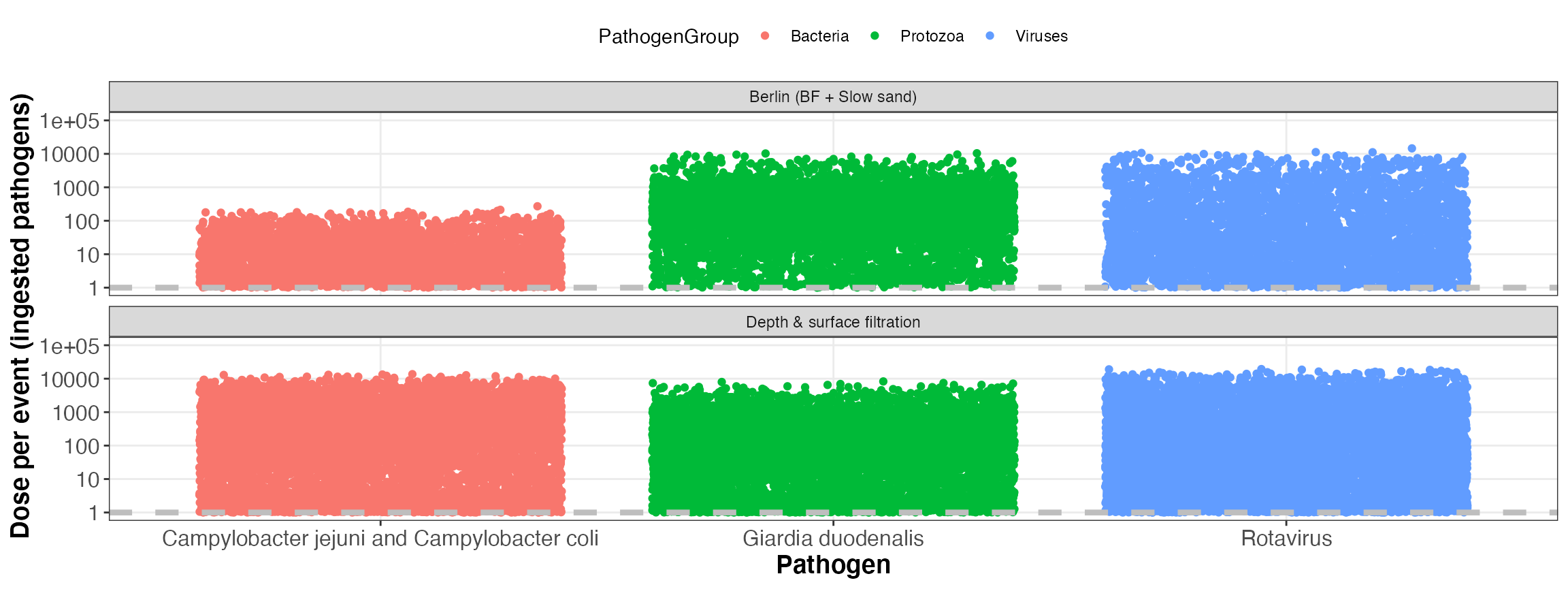
Simulated dose per event
kwb.qmra::plot_event_volume(risk)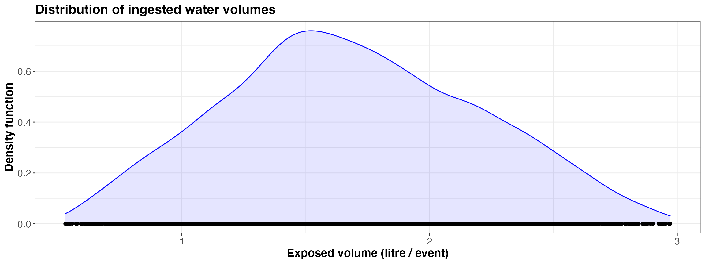
Simulated ingested volume per event
5.5 Health results
5.5.1 Per event
kwb.qmra::plot_event_infectionProb(risk)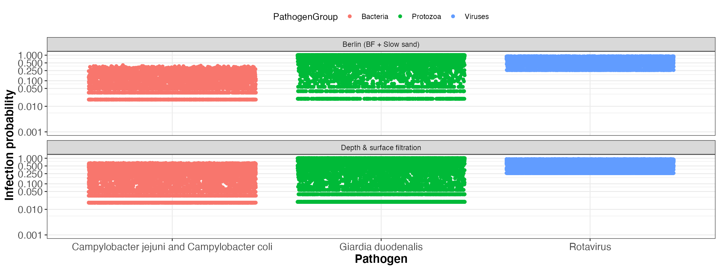
Simulated infection probability per event
kwb.qmra::plot_event_illnessProb(risk)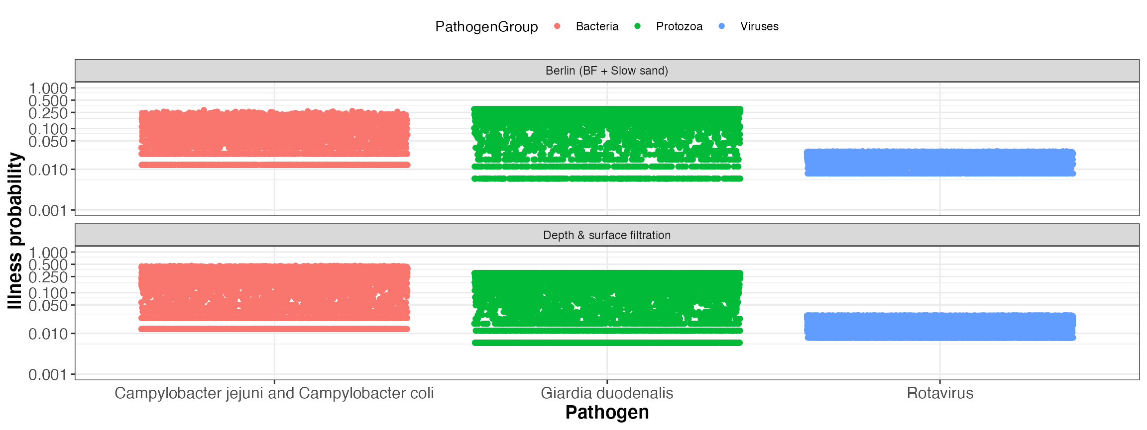
Simulated illness probability per event
kwb.qmra::plot_event_dalys(risk)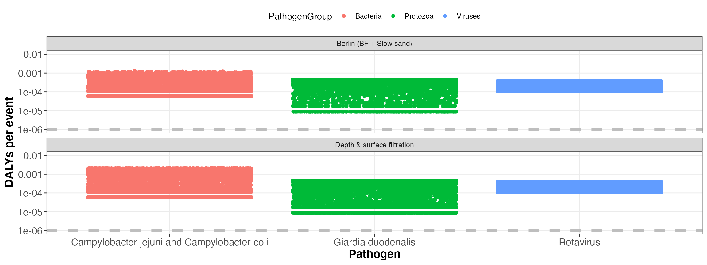
Simulated DALYs per event
5.5.2 Total
kwb.qmra::plot_total_infectionProb(risk)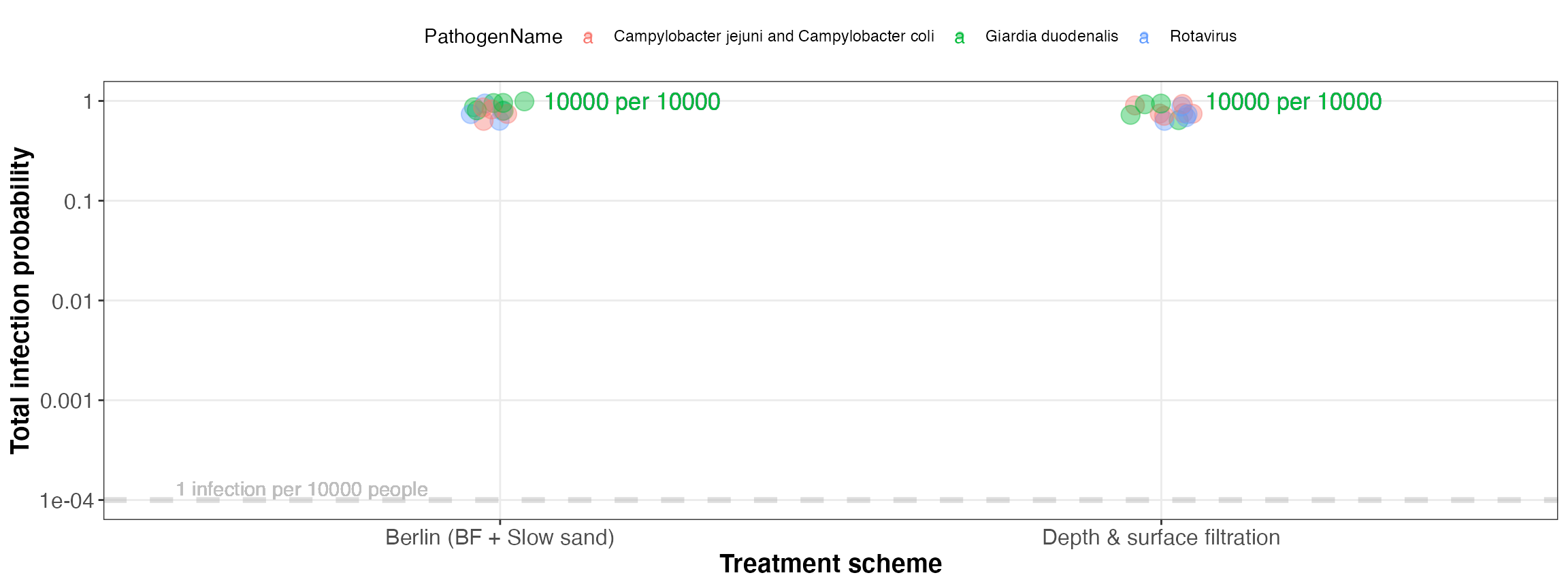
Simulated total infection probability (for all events)
kwb.qmra::plot_total_illnessProb(risk)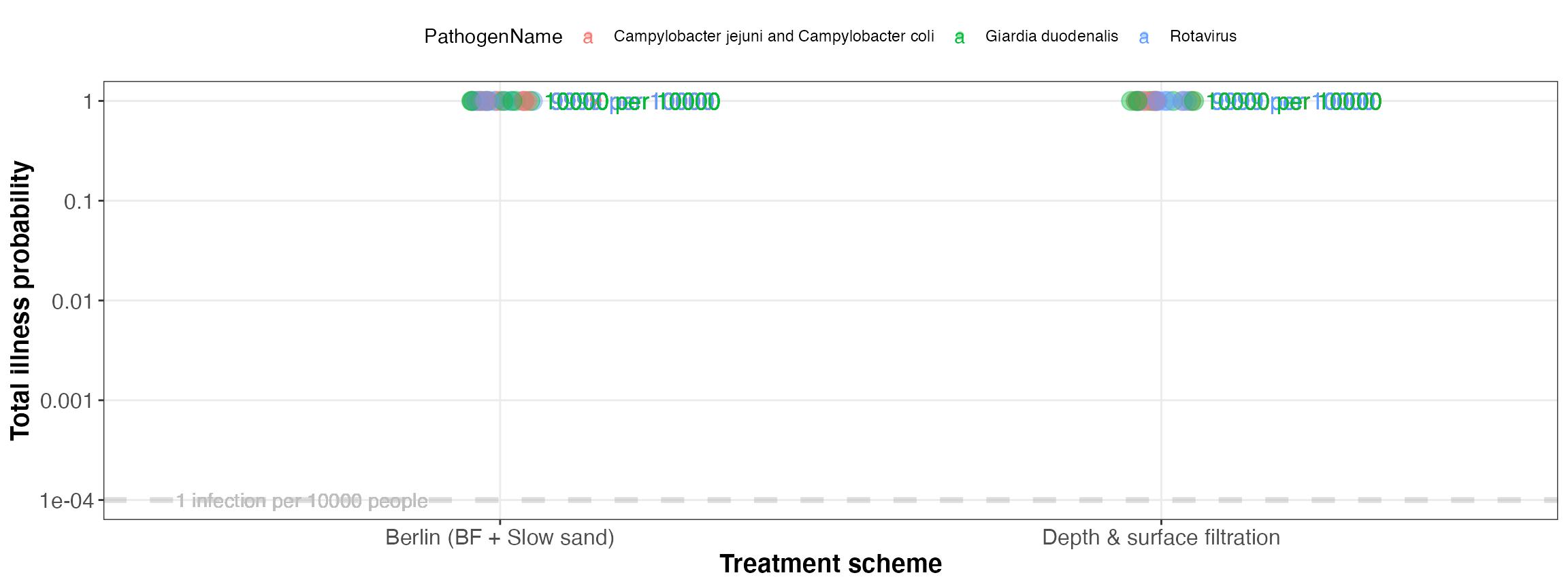
Simulated total illness probability (for all events
kwb.qmra::plot_total_dalys(risk)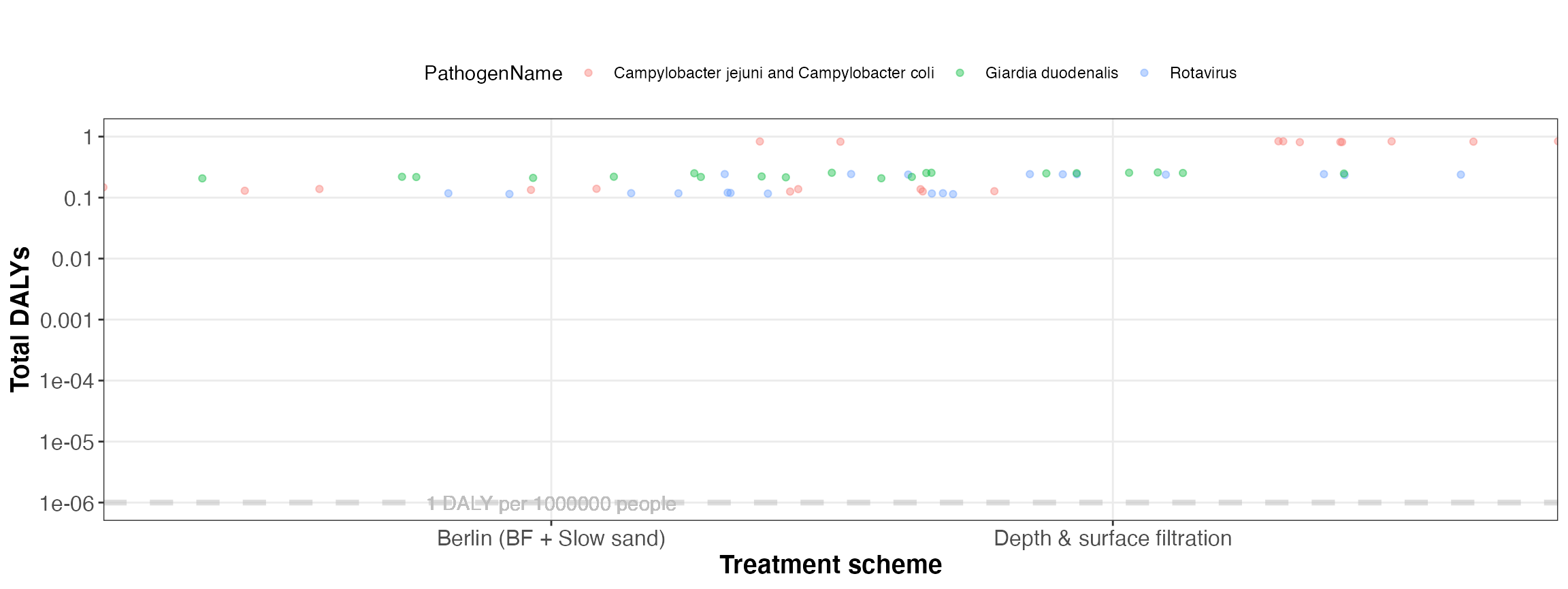
Simulated total DALYs (for all events)
In addtion tables with summary statistics, e.g. for the total risk can be generated easily as shown below:
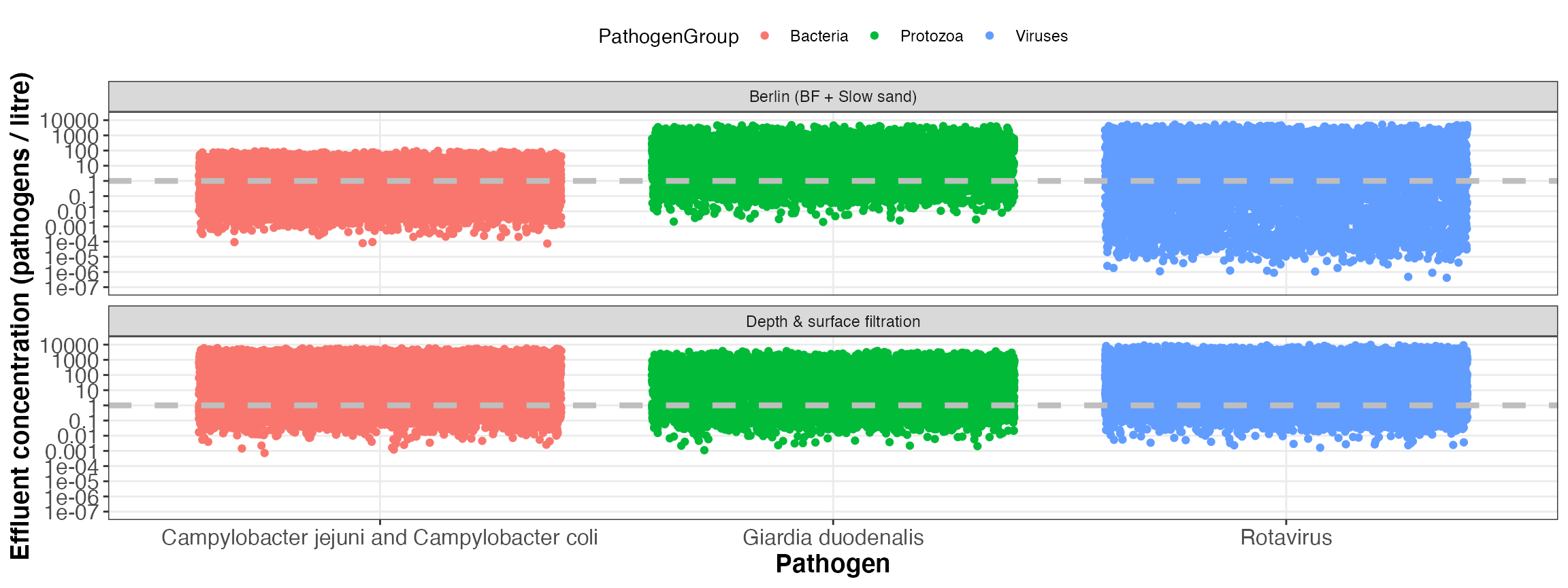
| repeatID | TreatmentSchemeID | TreatmentSchemeName | PathogenID | PathogenName | PathogenGroup | events | inflow_median | logreduction_median | volume_sum | exposure_sum | dose_sum | infectionProb_sum | illnessProb_sum | dalys_sum |
|---|---|---|---|---|---|---|---|---|---|---|---|---|---|---|
| 1 | 1 | Berlin (BF + Slow sand) | 3 | Campylobacter jejuni and Campylobacter coli | Bacteria | 730 | 4956.769 | 4.040410 | 1225.871 | 6148.256 | 6179 | 1 | 1.0000000 | 0.1295407 |
| 1 | 1 | Berlin (BF + Slow sand) | 32 | Rotavirus | Viruses | 730 | 4892.187 | 3.393638 | 1225.871 | 210089.734 | 210825 | 1 | 0.9997758 | 0.1164240 |
| 1 | 1 | Berlin (BF + Slow sand) | 36 | Giardia duodenalis | Protozoa | 730 | 5147.018 | 1.695504 | 1225.871 | 268234.677 | 268988 | 1 | 1.0000000 | 0.2181268 |
| 1 | 2 | Depth & surface filtration | 3 | Campylobacter jejuni and Campylobacter coli | Bacteria | 1095 | 4956.769 | 2.472764 | 1838.807 | 646691.655 | 646408 | 1 | 1.0000000 | 0.8165979 |
| 1 | 2 | Depth & surface filtration | 32 | Rotavirus | Viruses | 1095 | 4892.187 | 2.591457 | 1838.807 | 737878.955 | 736889 | 1 | 1.0000000 | 0.2380598 |
| 1 | 2 | Depth & surface filtration | 36 | Giardia duodenalis | Protozoa | 1095 | 5147.018 | 1.960714 | 1838.807 | 347994.659 | 347626 | 1 | 1.0000000 | 0.2557319 |
6 Export results
E.g. Write reports for all configurations in package subfolder extdata/configs/ (here: /Users/runner/work/_temp/Library/kwb.qmra/extdata/configs/):
confDirs <- system.file("extdata/configs/", package = "kwb.qmra")
kwb.qmra::report_workflow(confDirs)