Modelling with R: Status Quo (2017-05-01 - 2020-10-31)
Michael Rustler
Source:vignettes/modelling_r.Rmd
modelling_r.RmdThis workflow is based on using the R package kwb.hydrus1d, which is
compatible with the last official release of HYDRUS1D
v4.17.0140. The development of this new R package was
necessary, due to the fact that already available model wrappers were
developed for outdated HYDRUS1D versions (e.g. python
package phydrus
requires HYDRUS1D
v4.08) and/or are not well maintained (e.g. open issues/pull
requests for R package hydrusR).
The workflow below describes all the steps required for:
Input data preparation
Modifying (i.e.
atmosphericinput data defined in fileATMOSPHERE.in) an already pre-preparedHYDRUS1Dmodel (using theHYDRUS1D GUI)Running it from within
Rby using the command line (cmd) andImporting and analysing the
HYDRUS1Dresults within R.
Install R Package
# Enable this universe
options(repos = c(
  kwbr = 'https://kwb-r.r-universe.dev',
  CRAN = 'https://cloud.r-project.org'))
# Install R package
install.packages('flextreat.hydrus1d')
Define Paths
paths_list <- list(
  extdata = system.file("extdata", package = "flextreat.hydrus1d"),
  exe_dir = "<extdata>/model",
  scenario = "status-quo",
  model_name = "test",
  model_dir = "<exe_dir>/<model_name>",
  atmosphere = "<model_dir>/ATMOSPH.IN",
  a_level = "<model_dir>/A_LEVEL.out",
  t_level = "<model_dir>/T_LEVEL.out",
  runinf = "<model_dir>/Run_Inf.out",
  solute_id = 1,
  solute = "<model_dir>/solute<solute_id>.out",
  soil_data = "<extdata>/input-data/soil/soil_geolog.csv"
)

paths <- kwb.utils::resolve(paths_list)
Input Data
Soil
Soil data is derived from depth-dependent grain-size analysis of soil
samples taken in Braunschweig. The following required input parameters
for the van Genuchten model used in HYDRUS1D
were derived by using the pedotransfer function ROSETTA-API
version 3, which was developed by Zhang and Schaap,
2017.
library(flextreat.hydrus1d)

soil_dat <- readr::read_csv(paths$soil_data, show_col_types = FALSE) %>%
  dplyr::mutate(layer_id = dplyr::if_else(.data$tiefe_cm_ende < 60,
                                       1,
                                       2),
                thickness_cm = .data$tiefe_cm_ende - .data$tiefe_cm_start,
                sand = .data$S_prozent + .data$G_prozent,
                silt = .data$U_prozent,
                clay = round(100 - .data$sand - .data$silt,
                                     1)) %>%
  dplyr::mutate(clay = dplyr::if_else(.data$clay < 0,
                                      0,
                                      .data$clay)) %>%
  soilDB:::ROSETTA(vars = c("sand", "silt", "clay"),
                   v = "3") %>%
  dplyr::mutate(alpha = 10^.data$alpha,
                npar = 10^.data$npar,
                ksat = 10^.data$ksat)


knitr::kable(soil_dat)| tiefe_cm | tiefe_cm_start | tiefe_cm_ende | gluehverlust_prozent | U_prozent | S_prozent | G_prozent | kf_beyer | layer_id | thickness_cm | sand | silt | clay | theta_r | theta_s | alpha | npar | ksat | .rosetta.model | .rosetta.version |
|---|---|---|---|---|---|---|---|---|---|---|---|---|---|---|---|---|---|---|---|
| 0 - 30 | 0 | 30 | 2.7 | 6.4 | 93.1 | 0.4 | 9.5e-05 | 1 | 30 | 93.5 | 6.4 | 0.1 | 0.0481310 | 0.3671023 | 0.0334257 | 3.014652 | 716.3720 | 2 | 3 |
| 30 - 55 | 30 | 55 | 1.3 | 6.3 | 93.3 | 0.4 | 1.3e-04 | 1 | 25 | 93.7 | 6.3 | 0.0 | 0.0480175 | 0.3669818 | 0.0335768 | 3.053357 | 739.3399 | 2 | 3 |
| 55 - 80 | 55 | 80 | 0.6 | 1.7 | 97.3 | 1.1 | 1.9e-04 | 2 | 25 | 98.4 | 1.7 | 0.0 | 0.0485529 | 0.3626158 | 0.0355315 | 3.951321 | 1296.6154 | 2 | 3 |
| 80 - 150 | 80 | 150 | 0.2 | 1.3 | 98.6 | 0.1 | 2.0e-04 | 2 | 70 | 98.7 | 1.3 | 0.0 | 0.0486320 | 0.3621635 | 0.0356286 | 4.021821 | 1343.1455 | 2 | 3 |
| 150 - 190 | 150 | 190 | 0.2 | 1.0 | 98.7 | 0.3 | 2.2e-04 | 2 | 40 | 99.0 | 1.0 | 0.0 | 0.0486788 | 0.3618558 | 0.0357316 | 4.088764 | 1388.8655 | 2 | 3 |
| 190 - 210 | 190 | 210 | 0.3 | 2.5 | 97.2 | 0.3 | 1.7e-04 | 2 | 20 | 97.5 | 2.5 | 0.0 | 0.0484589 | 0.3633709 | 0.0351930 | 3.764078 | 1171.5976 | 2 | 3 |
Due to similar soil characteristics, only two different layers
(column layer_id) were defined: - layer 1:
ranging from 0 cm - 55 cm depth -
layer 2: ranging from 55 cm -
210 cm depth
The spatially aggregation for each layer (geometric mean) of the
input parameters for the van Genuchten model is performed
with the code below and shown in the subsequent table.
soil_dat_per_layer <- soil_dat %>%
  dplyr::group_by(.data$layer_id) %>%
  dplyr::summarise(layer_thickness = max(.data$tiefe_cm_ende) - min(.data$tiefe_cm_start),
                   theta_r = sum(.data$theta_r*.data$thickness_cm)/.data$layer_thickness,
                   theta_s = sum(.data$theta_s*.data$thickness_cm)/.data$layer_thickness,
                   alpha = sum(.data$alpha*.data$thickness_cm)/.data$layer_thickness,
                   npar = sum(.data$npar*.data$thickness_cm)/.data$layer_thickness,
                   ksat = sum(.data$ksat*.data$thickness_cm)/.data$layer_thickness)


knitr::kable(soil_dat_per_layer)| layer_id | layer_thickness | theta_r | theta_s | alpha | npar | ksat |
|---|---|---|---|---|---|---|
| 1 | 55 | 0.0480794 | 0.3670475 | 0.0334944 | 3.032245 | 726.812 |
| 2 | 155 | 0.0486090 | 0.3623128 | 0.0355833 | 3.994469 | 1325.304 |
Atmospheric Boundary Conditions
In total three different atmospheric input boundary conditions
(precipitation, potential evaporation and
irrigation) are used within the HYDRUS1D model
and described in the following subchapters in more detail.
Rainfall
Rainfall is based on historical hourly raw data
downloaded from DWD
open-data ftp server for station_id = 662
(i.e. Braunschweig). Data is aggregated within R to daily
sums by using the code below:
install.packages("rdwd")
library(dplyr)
rdwd::updateRdwd()

rdwd::findID("Braunschweig")
rdwd::selectDWD(name = "Braunschweig", res = "daily")

url_bs_rain <- rdwd::selectDWD(name = "Braunschweig",
                               res = "hourly",
                               var = "precipitation",
                               per = "historical" )

bs_rain <- rdwd::dataDWD(url_bs_rain)

precipitation_hourly <- rdwd::dataDWD(url_bs_rain) %>%
  dplyr::select(.data$MESS_DATUM, .data$R1) %>%
  dplyr::rename("datetime" = "MESS_DATUM",
                "precipitation_mm" = "R1")

usethis::use_data(precipitation_hourly)


precipitation_daily <- precipitation_hourly %>%
  dplyr::mutate("date" = as.Date(datetime)) %>%
  dplyr::group_by(date) %>%
  dplyr::summarise(rain_mm = sum(precipitation_mm))

usethis::use_data(precipitation_daily)
DT::datatable(head(flextreat.hydrus1d::precipitation_daily))Potential Evaporation
Is based on daily potential evaporation grids (1km x
1km) downloaded from DWD
open-data server, where all grids (i.e. 46) within the
Abwasserverregnungsgebiet.shp were selected and spatially
aggregated (mean, sd, min,
max) by using the code below:
shape_file <- system.file("extdata/input-data/gis/Abwasserverregnungsgebiet.shp",
                          package = "flextreat.hydrus1d")

# Only data of full months can currently be read!
evapo_p <- kwb.dwd::read_daily_data_over_shape(
  file = shape_file,
  variable = "evapo_p",
  from = "201701",
  to = "202012"
)

usethis::use_data(evapo_p)Irrigation
Monthly irrigation volumes were provided by Abwasserverband
Braunschweig for the time period 2017-01-01 - 2023-12-31 as
csv file and separates between two sources
(groundwater and clearwater). Data preparation
was carried out with the code below:
irrigation_file <- system.file("extdata/input-data/Beregnungsmengen_AVB.csv",
                          package = "flextreat.hydrus1d")


# irrigation_area <- rgdal::readOGR(dsn = shape_file)
# irrigation_area_sqm <- irrigation_area$area  # 44111068m2

## 2700ha (https://www.abwasserverband-bs.de/de/was-wir-machen/verregnung/)
irrigation_area_sqm <- 27000000

irrigation <- read.csv2(irrigation_file) %>%
  dplyr::select(- .data$Monat) %>%
  dplyr::rename(irrigation_m3 = .data$Menge_m3,
                source = .data$Typ,
                month = .data$Monat_num,
                year = .data$Jahr) %>%
  dplyr::mutate(date_start = as.Date(sprintf("%d-%02d-01",
                               .data$year,
                               .data$month)),
                days_in_month = as.numeric(lubridate::days_in_month(.data$date_start)),
                date_end =  as.Date(sprintf("%d-%02d-%02d",
                                            .data$year,
                                            .data$month,
                                            .data$days_in_month)),
                source = kwb.utils::multiSubstitute(.data$source,
                                                    replacements = list("Grundwasser" = "groundwater.mmPerDay",
                                                                        "Klarwasser" = "clearwater.mmPerDay")),
                irrigation_cbmPerDay = .data$irrigation_m3/.data$days_in_month,
                irrigation_area_sqm = irrigation_area_sqm,
                irrigation_mmPerDay = 1000*irrigation_cbmPerDay/irrigation_area_sqm) %>%
  dplyr::select(.data$year,
                .data$month,
                .data$days_in_month,
                .data$date_start,
                .data$date_end,
                .data$source,
                .data$irrigation_mmPerDay,
                .data$irrigation_area_sqm) %>%
  tidyr::pivot_wider(names_from = .data$source,
                     values_from = .data$irrigation_mmPerDay)


usethis::use_data(irrigation)
DT::datatable(head(flextreat.hydrus1d::irrigation))HYDRUS-1D
Modify Input Files
All model input files were initially setup by using the
HYDRUS1D-GUI but the following below were modified manually
with the
SELECTOR.in
Soil input data were entered manually in SELECTOR.in for
the two layers defined the second table in Chapter:
Input Data - Soil.
ATMOSPHERE.in
Based on the atmospheric input data (see Chapter: Atmospheric Boundary
Conditions) the ATMOSPHERE.in file for
HYDRUS1D is prepared with the code below and starts with
the hydrological summer half year (assumption: soil is
fully wetted at end of winter half year):
atm <- flextreat.hydrus1d::prepare_atmosphere_data()
atm_selected <- flextreat.hydrus1d::select_hydrologic_years(atm)

atm_selected_hydro_wide <- flextreat.hydrus1d::aggregate_atmosphere(atm_selected, "wide")

DT::datatable(atm_selected_hydro_wide)
atm_selected_hydro_long <- flextreat.hydrus1d::aggregate_atmosphere(atm_selected, "long")

atm_hydro_plot <- flextreat.hydrus1d::plot_atmosphere(atm_selected_hydro_long)
atm_hydro_plot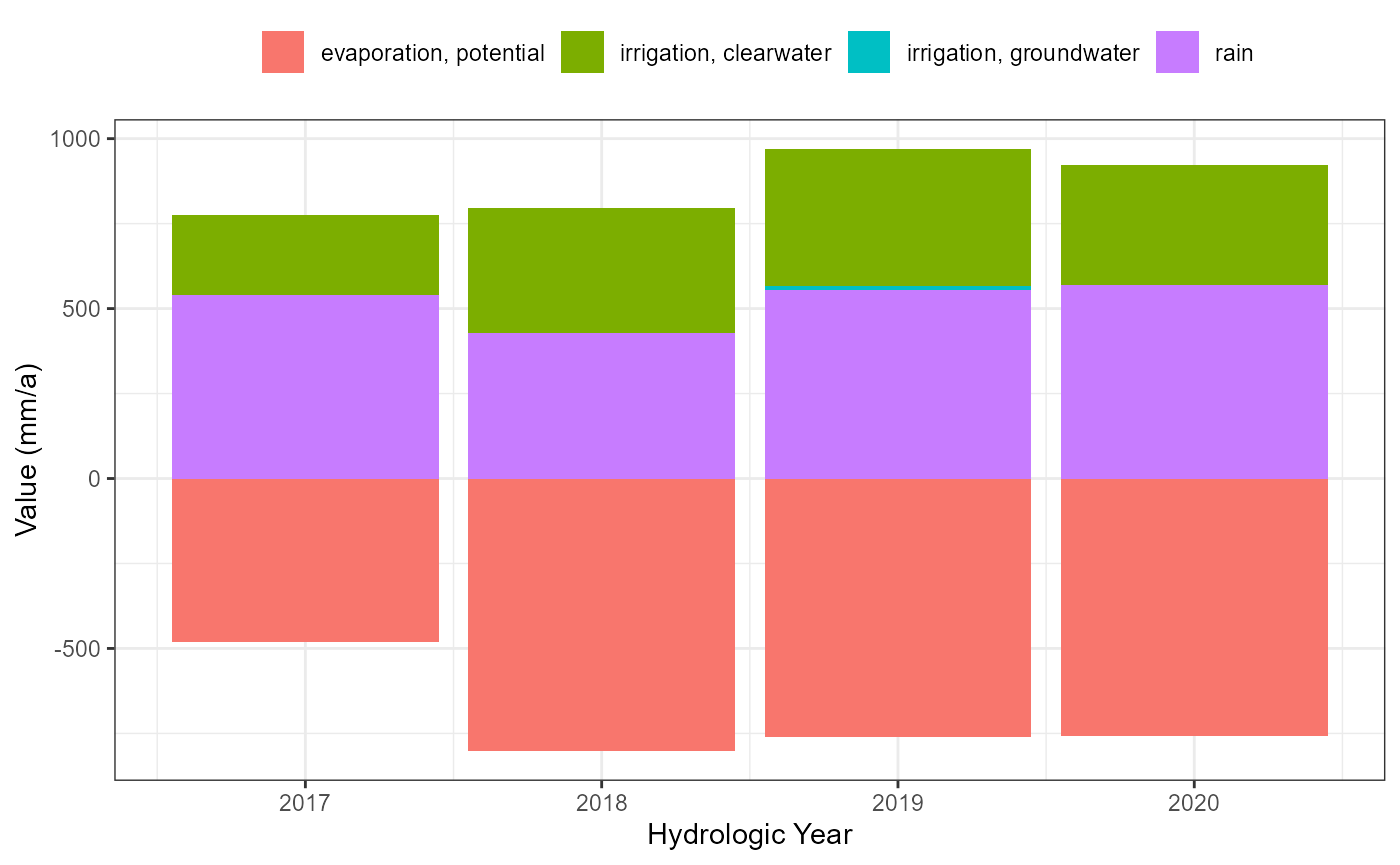
kwb.utils::preparePdf(pdfFile = sprintf("boundaries-temporal_%s.pdf",
                                        paths$scenario),
                                        width.cm = 18, height.cm = 10)
#> [1] "boundaries-temporal_status-quo.pdf"
atm_hydro_plot
dev.off()
#> agg_png
#>       2


atm_prep <- flextreat.hydrus1d::prepare_atmosphere(
  atm_selected,
  conc_irrig_clearwater = 1, # use as "clearwater" tracer
  conc_irrig_groundwater = 0,
  conc_rain = 0)

atmos <- kwb.hydrus1d::write_atmosphere(
  atm = atm_prep,
  MaxAL = nrow(atm_prep),
  round_digits = 6 # increase precision for "clearwater" tracer!
  )

writeLines(atmos, paths$atmosphere)
The selected time period covers 2374 days (2017-05-01 - 2023-10-31), i.e. it covers 13 hydrological half years.
DT::datatable(atm_selected)These time-series were converted with the function
flextreat.hydrus1d::prepare_atmosphere() into the data
format required by HYDRUS1D. Due to the fact, that
irrigation rates (i.e. sum of
clearwater.mmPerDay and groundwater.mmPerDay)
cannot be entered separately as input column within
HYDRUS1D, these were simply added to th prec
(i.e. precipitation) column. The whole time series defined
in ATMOSPHERE.in is shown below:
DT::datatable(atm_prep)Run Model
Finally the model is run automatically by using the following code:
exe_path <- kwb.hydrus1d::check_hydrus_exe(dir = paths$exe_dir,
                                           skip_preinstalled = TRUE)
#> Checking if download of HYDRUS1D executable v4.17.0140 from 'https://github.com/mrustl/hydrus1d/archive/refs/tags/v4.17.0140.zip' was successful ... ok. (0.00 secs)
kwb.hydrus1d:::run_model(exe_path = exe_path,
                         model_path = paths$model_dir)
#> Warning in shell(cmd = sprintf("cd %s && %s", fs::path_abs(target_dir), : 'cd
#> D:/a/_temp/Library/flextreat.hydrus1d/extdata/model && H1D_CALC.exe' execution
#> failed with error code 24
Read Results
Numerical Solution
runinf <- kwb.hydrus1d::read_runinf(paths$runinf)

summary(runinf)
#>     t_level           time               dt               itr_w
#>  Min.   :    1   Min.   :   0.05   Min.   :0.001525   Min.   : 2.000
#>  1st Qu.: 5595   1st Qu.: 297.29   1st Qu.:0.025572   1st Qu.: 2.000
#>  Median :11188   Median : 629.35   Median :0.055000   Median : 2.000
#>  Mean   :11188   Mean   : 622.06   Mean   :0.057159   Mean   : 2.454
#>  3rd Qu.:16782   3rd Qu.: 953.83   3rd Qu.:0.096046   3rd Qu.: 2.000
#>  Max.   :22376   Max.   :1279.00   Max.   :0.100000   Max.   :20.000
#>      itr_c       it_cum          kod_t             kod_b    converg
#>  Min.   :1   Min.   :    3   Min.   :-4.0000   Min.   :-5   Mode:logical
#>  1st Qu.:1   1st Qu.:17337   1st Qu.:-4.0000   1st Qu.:-5   TRUE:22376
#>  Median :1   Median :33876   Median :-4.0000   Median :-5
#>  Mean   :1   Mean   :34340   Mean   :-0.7447   Mean   :-5
#>  3rd Qu.:1   3rd Qu.:50978   3rd Qu.: 4.0000   3rd Qu.:-5
#>  Max.   :1   Max.   :68153   Max.   : 4.0000   Max.   :-5
#>      peclet       courant
#>  Min.   :0.1   Min.   :0.00100
#>  1st Qu.:0.1   1st Qu.:0.02100
#>  Median :0.1   Median :0.05500
#>  Mean   :0.1   Mean   :0.09919
#>  3rd Qu.:0.1   3rd Qu.:0.14600
#>  Max.   :0.1   Max.   :0.98400
Conservative Tracer
solute <- kwb.hydrus1d::read_solute(paths$solute)

solute_date <- flextreat.hydrus1d::aggregate_solute(solute,
                                                    col_aggr = "date")
solute_yearmonth <- flextreat.hydrus1d::aggregate_solute(solute,
                                                         col_aggr = "yearmonth")
solute_year_hydrologic <- flextreat.hydrus1d::aggregate_solute(solute,
                                                               col_aggr = "year_hydrologic") %>%
  dplyr::filter(.data$diff_time >= 364) ### filter out as only may-october

DT::datatable(solute_year_hydrologic)
solute_date_plot <- flextreat.hydrus1d::plot_solute(solute_date)
solute_yearmonth_plot <- flextreat.hydrus1d::plot_solute(solute_yearmonth)

solute_date_plot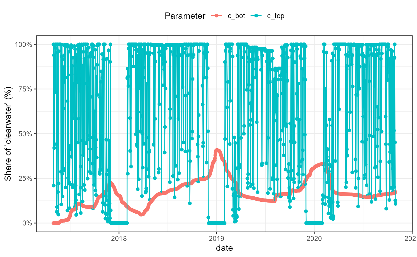
solute_yearmonth_plot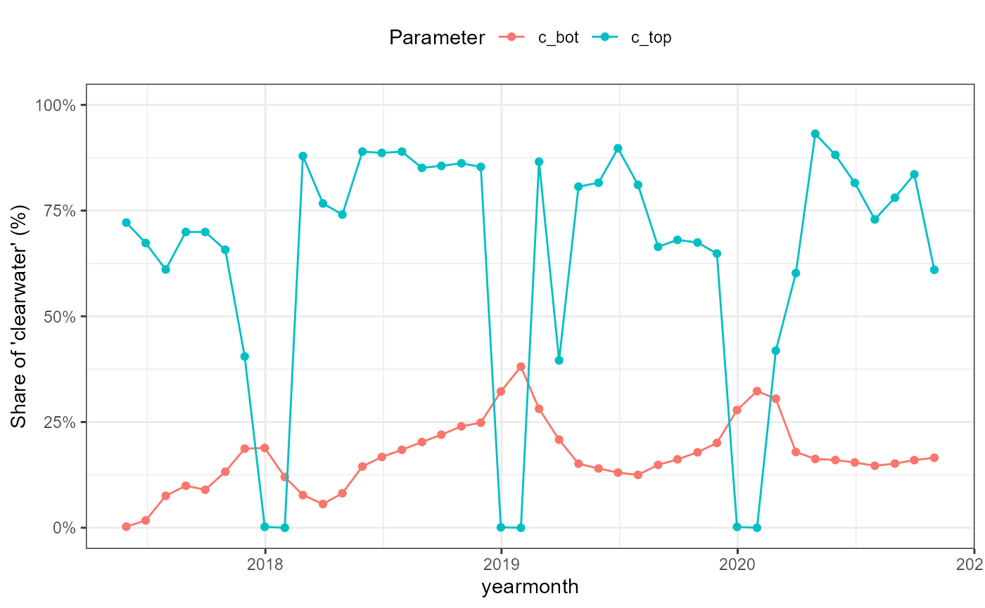
kwb.utils::preparePdf(pdfFile = sprintf("solute_yearmonth_%s.pdf",
                                        paths$scenario),
                      width.cm = 22,
                      height.cm = 10)
#> [1] "solute_yearmonth_status-quo.pdf"
solute_yearmonth_plot
dev.off()
#> agg_png
#>       2
Water Balance
t_level <- kwb.hydrus1d::read_tlevel(paths$t_level)
t_level
#> # A tibble: 22,376 × 22
#>     time r_top r_root  v_top v_root    v_bot sum_r_top sum_r_root sum_v_top
#>  * <dbl> <dbl>  <dbl>  <dbl>  <dbl>    <dbl>     <dbl>      <dbl>     <dbl>
#>  1 0.05  0.134      0 0.134       0 -0.00173   0.00668          0   0.00668
#>  2 0.1   0.134      0 0.134       0 -0.00173   0.0134           0   0.0134
#>  3 0.155 0.134      0 0.134       0 -0.00173   0.0207           0   0.0207
#>  4 0.216 0.134      0 0.134       0 -0.00173   0.0288           0   0.0288
#>  5 0.282 0.134      0 0.134       0 -0.00173   0.0377           0   0.0377
#>  6 0.354 0.134      0 0.134       0 -0.00173   0.0473           0   0.0473
#>  7 0.381 0.134      0 0.0874      0 -0.00173   0.0509           0   0.0496
#>  8 0.410 0.134      0 0.0652      0 -0.00173   0.0548           0   0.0516
#>  9 0.421 0.134      0 0.0507      0 -0.00173   0.0563           0   0.0521
#> 10 0.433 0.134      0 0.0516      0 -0.00173   0.0579           0   0.0527
#> # ℹ 22,366 more rows
#> # ℹ 13 more variables: sum_v_root <dbl>, sum_v_bot <dbl>, h_top <dbl>,
#> #   h_root <dbl>, h_bot <dbl>, run_off <dbl>, sum_run_off <dbl>, volume <dbl>,
#> #   sum_infil <dbl>, sum_evap <dbl>, t_level <dbl>, cum_w_trans <dbl>,
#> #   snow_layer <dbl>

## t_level aggregate
tlevel_aggr_date <- flextreat.hydrus1d::aggregate_tlevel(t_level)
tlevel_aggr_yearmonth <- flextreat.hydrus1d::aggregate_tlevel(t_level,
                                                              col_aggr = "yearmonth")
tlevel_aggr_year_hydrologic <- flextreat.hydrus1d::aggregate_tlevel(t_level,
                                                                    col_aggr = "year_hydrologic") %>%
  dplyr::filter(.data$diff_time >= 364) ### filter out as only may-october

DT::datatable(tlevel_aggr_year_hydrologic)
wb_date_plot <- flextreat.hydrus1d::plot_waterbalance(tlevel_aggr_date)
wb_yearmonth_plot <- flextreat.hydrus1d::plot_waterbalance(tlevel_aggr_yearmonth)
wb_yearhydrologic_plot <- flextreat.hydrus1d::plot_waterbalance(tlevel_aggr_year_hydrologic)

wb_date_plot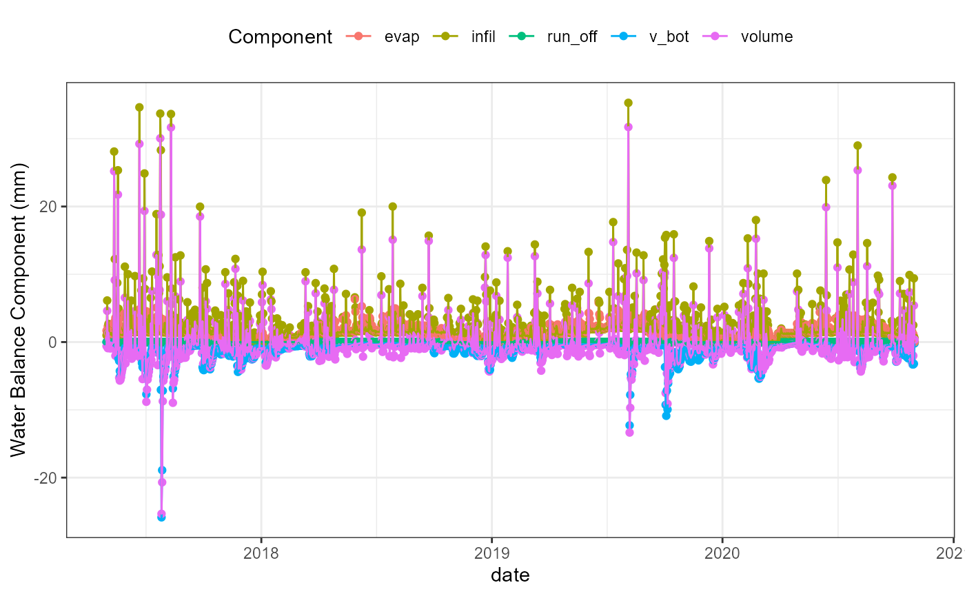
wb_yearmonth_plot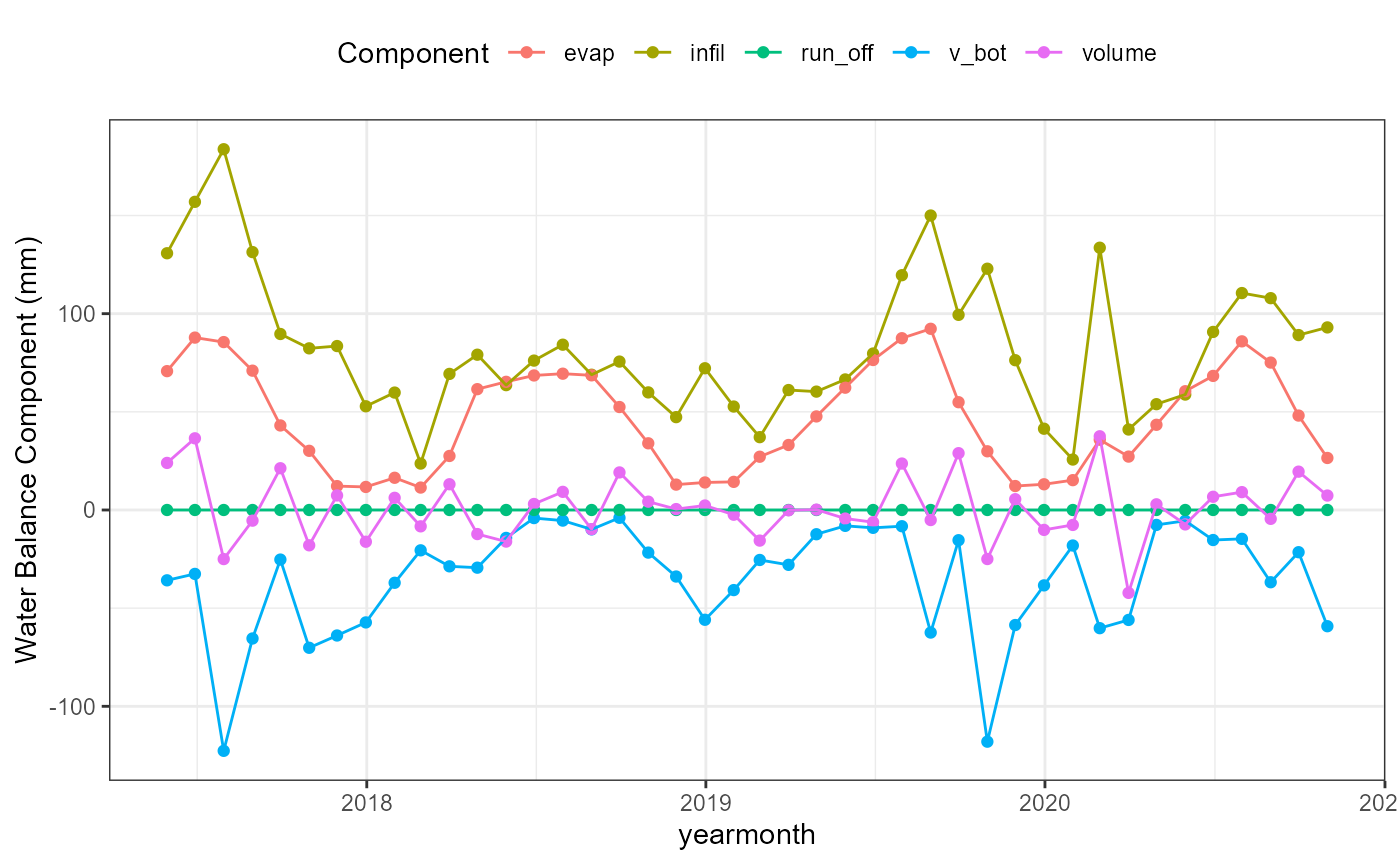
wb_yearhydrologic_plot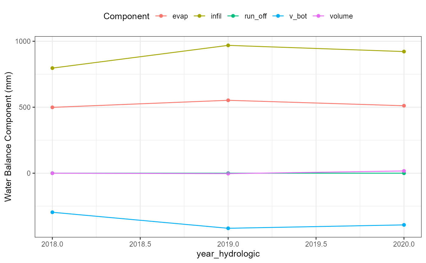
kwb.utils::preparePdf(pdfFile = sprintf("water-balance_yearmonth_%s.pdf",
                                        paths$scenario),
                                        width.cm = 19, height.cm = 10)
#> [1] "water-balance_yearmonth_status-quo.pdf"
wb_yearmonth_plot
dev.off()
#> agg_png
#>       2

saveRDS(wb_yearmonth_plot,
        file = sprintf("wb_yearmonth_%s.Rds", paths$scenario))
plotly::ggplotly(wb_date_plot)
plotly::ggplotly(wb_yearmonth_plot)
a_level <- kwb.hydrus1d::read_alevel(paths$a_level)
a_level
#> # A tibble: 1,279 × 10
#>     time sum_r_top sum_r_root sum_v_top sum_v_root sum_v_bot     h_top h_root
#>  * <dbl>     <dbl>      <dbl>     <dbl>      <dbl>     <dbl>     <dbl>  <dbl>
#>  1     1  0.134             0    0.0686          0  -0.00173 -100000        0
#>  2     2 -0.336             0   -0.401           0  -0.00346     -82.5      0
#>  3     3 -0.230             0   -0.295           0  -0.00520    -161.       0
#>  4     4 -0.369             0   -0.434           0  -0.00693     -97.5      0
#>  5     5 -0.351             0   -0.416           0  -0.00866    -122.       0
#>  6     6 -0.210             0   -0.290           0  -0.0104  -100000        0
#>  7     7 -0.104             0   -0.256           0  -0.0121  -100000        0
#>  8     8 -0.113             0   -0.265           0  -0.0139     -185.       0
#>  9     9 -0.000812          0   -0.222           0  -0.0156  -100000        0
#> 10    10  0.182             0   -0.206           0  -0.0173  -100000        0
#> # ℹ 1,269 more rows
#> # ℹ 2 more variables: h_bot <dbl>, a_level <dbl>