Installation
### Optionally: specify GitHub Personal Access Token (GITHUB_PAT)
### See here why this might be important for you:
### https://kwb-r.github.io/kwb.pkgbuild/articles/install.html#set-your-github_pat

# Sys.setenv(GITHUB_PAT = "mysecret_access_token")

# Install package "remotes" from CRAN
if (! require("remotes")) {
  install.packages("remotes", repos = "https://cloud.r-project.org")
}

# Install KWB package 'kwb.heatsine' from GitHub
remotes::install_github("KWB-R/kwb.heatsine")
Data prerequisites
The sinus fit optimisation works for daily time series of a surface water and a groundwater monitoring point, which follow the following requirements:
File naming
The time series must be provided in a .csv (comma separated value) file, which follows the naming convention:
temperature_<type>_<monitoring_id>.csv
where <type> needs to be exactly groundwater or surface-water. In case any other value for <type> is chosen the program will not work (e.g SURFACE WATER). The value of the <monitoring_id> will be used for labeling the monitoring points in the plots and can be almost any value but must not contain _ (underscore) or " " (space).
Data structure
The data structure of each .csv file is very simple as it contains only the two columns date (formatted: YYYY-MM-DD, e.g. 2020-06-23) and value (temperature data in degree Celsius) as shown exemplary below:
Please make sure that both columns date and value are all lowercase and correctly spelled as the program will not work if this is not the case.
Data preparation
Import
The R package includes the following temporal times series data for testing:
list.files(kwb.heatsine::extdata_file())
#> [1] "temperature_groundwater_Txxbxxxx6.csv"
#> [2] "temperature_groundwater_Txxhxxx10.csv"
#> [3] "temperature_groundwater_Txxsxxx20.csv"
#> [4] "temperature_groundwater_Txxwxxx13.csv"
#> [5] "temperature_groundwater_Txxxx3.csv"
#> [6] "temperature_surface-water_Txxsxx-mxxxxsxxx.csv"
In this the example the files temperature_surface-water_Txxsxx-mxxxxsxxx.csv and temperature_groundwater_Txxxx3.csv are used for testing the functionality and imported by using the code below:
## Load the R package
library(kwb.heatsine)

load_temp <- function(base_name) {
  kwb.heatsine::load_temperature_from_csv(
    kwb.heatsine::extdata_file(base_name)
  )
}

data_sw <- load_temp("temperature_surface-water_Txxsxx-mxxxxsxxx.csv")
data_gw <- load_temp("temperature_groundwater_Txxxx3.csv")
Visualise
Plot time series for whole time period (moveover on data points to select)
Surface water
kwb.heatsine::plot_temperature_interactive(data_sw)
Groundwater
kwb.heatsine::plot_temperature_interactive(data_gw)
Select
Reduce time period to a full sinus period which is definde by the user input (date_end is optional, if not given it is set to ‘date_start’ + 365.25 days).
data_sw_selected <- kwb.heatsine::select_timeperiod(
  data_sw,
  date_start = "2015-10-10",
  date_end = "2016-10-14"
)

data_gw_selected <- kwb.heatsine::select_timeperiod(
  data_gw,
  date_start = "2015-12-28",
  date_end = "2016-12-26"
)
Plot selected datasets:
Surface Water (selected)
kwb.heatsine::plot_temperature_interactive(df = data_sw_selected)
Grundwater (selected)
kwb.heatsine::plot_temperature_interactive(df = data_gw_selected)
Sinus optimisation
Background
According to Cross Validated (2013) the sinus fit can not only be written as y = y0 + amplitude * sin(x + phase_shift), but also in a linear form y = y0 + alpha * sin(x) + beta * cos(x). The latter approach is used within this R package as it enables the calculation of both amplitude (a) and phase_shift (x0) by using R’s build-in stats::lm() function as exemplary shown below:
### Generate synthetic temperature data following sine curve


period_length <- 365 # assumed period length
day_number <- seq_len(period_length) # daily sequence from 1 to period_length
temperature <- 26.9188 + 2.123641 * sin(2 * pi * day_number / period_length + 0.6049163)

x <- 2 * pi * day_number / period_length

### Print first data points:
tibble::tibble(day_number = day_number, temperature = temperature, x = x)
#> # A tibble: 365 x 3
#>    day_number temperature      x
#>         <int>       <dbl>  <dbl>
#>  1          1        28.2 0.0172
#>  2          2        28.2 0.0344
#>  3          3        28.2 0.0516
#>  4          4        28.2 0.0689
#>  5          5        28.3 0.0861
#>  6          6        28.3 0.103
#>  7          7        28.3 0.120
#>  8          8        28.4 0.138
#>  9          9        28.4 0.155
#> 10         10        28.4 0.172
#> # … with 355 more rows

### Now check the if both formulas yield (almost) equal results

fit.lm2 <- lm(temperature ~ sin(x) + cos(x))

coeffs <- coef(fit.lm2)

y0 <- coeffs[1L] # y0
alpha <- coeffs[2L] # alpha = sin(phi)
beta <- coeffs[3L]  # beta = cos(phi)
a <- sqrt(alpha ^ 2 + beta ^ 2) # amplitude
x0 <- atan2(beta, alpha) # phase t

### Print parameters of sinus fit
tibble::tibble(
  y0 = y0,
  alpha = alpha,
  beta = beta,
  a = a,
  x0 = x0
)
#> # A tibble: 1 x 5
#>      y0 alpha  beta     a    x0
#>   <dbl> <dbl> <dbl> <dbl> <dbl>
#> 1  26.9  1.75  1.21  2.12 0.605

x <- 2 * pi * day_number / period_length

par(mfrow = c(1, 2))

### Formula option 1: y = y0 + amplitude * sin(x + phase)
plot(
  x = day_number,
  y = y0 + a * sin(x + x0),
  type = "l",
  lty = 1,
  lwd = 3,
  col = "gray",
  main = "Overplotted Graphs",
  xlab = "day_number",
  ylab = "temperature"
)

### Formula option 2: y = y0 + alpha * sin(x) + beta * cos(x)

lines(
  x = day_number,
  y = y0 + alpha * sin(x) + beta * cos(x),
  lwd = 2,
  lty = 2,
  col = "red",
)

### Check numeric differences between both approaches
plot(
  x = day_number,
  y = y0 + a * sin(x + x0) - (y0 + alpha * sin(x) + beta * cos(x)),
  lwd = 3,
  col = "gray",
  main = "Difference",
  xlab = "day_number",
  ylab = "temperature"
)
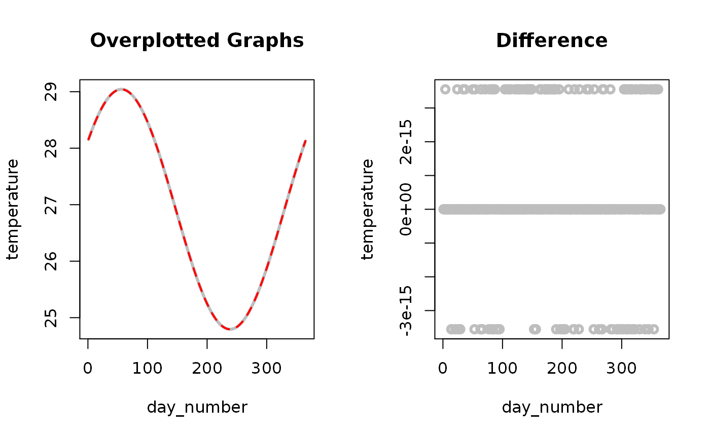
As shown above the differences between both sinus calculation approaches are mostly zero but sometimes show a minimal offset (which is close to R’s floating point accuracy of 10^-15.6535598 , i.e. 2.22044610^{-16} for the machine the calculation was carried out). As a consequence the second approach can and will be used for sinus fitting within this R package.
Run
Sinus fit operation is performed by minimizing the RMSE error between observed and simulated temperature curves.
# Generate data frame with simulated and observed values
predictions <- kwb.heatsine::run_optimisation(data_sw_selected,
                                              data_gw_selected,
                                              retardation_factor = 1.8
                                              )
Analyse
Interactive Plot
kwb.heatsine::plot_prediction_interactive(predictions)
#> Warning: `group_by_()` is deprecated as of dplyr 0.7.0.
#> Please use `group_by()` instead.
#> See vignette('programming') for more help
#> This warning is displayed once every 8 hours.
#> Call `lifecycle::last_warnings()` to see where this warning was generated.
Table: Traveltimes
knitr::kable(predictions$traveltimes)
| point_type | surface-water (Txxsxx-mxxxxsxxx) | groundwater (Txxxx3) | traveltime_thermal_days | retardation_factor | traveltime_hydraulic_days |
|---|---|---|---|---|---|
| turning-point_1 | 2015-10-21 | 2016-01-11 | 82.12867 | 1.8 | 45.62704 |
| min | 2016-01-23 | 2016-04-14 | 82.00000 | 1.8 | 45.55556 |
| turning-point_2 | 2016-04-25 | 2016-07-16 | 81.87133 | 1.8 | 45.48407 |
| max | 2016-07-28 | 2016-10-18 | 82.00000 | 1.8 | 45.55556 |
| turning-point_3 | 2016-10-29 | 2017-01-19 | 81.87133 | 1.8 | 45.48407 |
Table: Goodness of Fit
While only RMSE is used for optimising the sinus fit, a number of goodness-of-fit parameters is also calculated and shown in the table below. For details on each of these parameters the use is referred to the function hydroGOF::gof() which is used for calculating all these values.
knitr::kable(predictions$gof)
| type | ME | MAE | MSE | RMSE | NRMSE % | PBIAS % | RSR | rSD | NSE | mNSE | rNSE | d | md | rd | cp | r | R2 | bR2 | KGE | VE |
|---|---|---|---|---|---|---|---|---|---|---|---|---|---|---|---|---|---|---|---|---|
| surface-water | 0 | 1.24 | 2.33 | 1.53 | 20.1 | 0 | 0.20 | 0.98 | 0.96 | 0.82 | -0.17 | 0.99 | 0.91 | 0.7 | -10.49 | 0.98 | 0.96 | 0.95 | 0.97 | 0.90 |
| groundwater | 0 | 0.24 | 0.12 | 0.35 | 12.5 | 0 | 0.13 | 0.99 | 0.98 | 0.90 | 0.99 | 1.00 | 0.95 | 1.0 | -23.85 | 0.99 | 0.98 | 0.98 | 0.99 | 0.98 |
Table: Optimisation Parameters
knitr::kable(predictions$paras)
| type | period_length | alpha | beta | y0 | a | x0 |
|---|---|---|---|---|---|---|
| surface-water | 373.5143 | -10.278478 | 2.0304625 | 12.72494 | 10.477113 | 2.946559 |
| groundwater | 372.9996 | -3.742912 | 0.9567905 | 10.73679 | 3.863268 | 2.891325 |
Table: Data
| type | monitoring_id | label | date | observed | simulated | residuals | simulated_pi_lower | simulated_pi_upper |
|---|---|---|---|---|---|---|---|---|
| surface-water | Txxsxx-mxxxxsxxx | surface-water (Txxsxx-mxxxxsxxx) | 2015-10-10 | 13.50958 | 14.75541 | -1.245822 | 11.72751 | 17.78331 |
| surface-water | Txxsxx-mxxxxsxxx | surface-water (Txxsxx-mxxxxsxxx) | 2015-10-11 | 12.88167 | 14.58222 | -1.700557 | 11.55433 | 17.61012 |
| surface-water | Txxsxx-mxxxxsxxx | surface-water (Txxsxx-mxxxxsxxx) | 2015-10-12 | 12.17833 | 14.40852 | -2.230183 | 11.38062 | 17.43642 |
| surface-water | Txxsxx-mxxxxsxxx | surface-water (Txxsxx-mxxxxsxxx) | 2015-10-13 | 11.68292 | 14.23433 | -2.551416 | 11.20643 | 17.26223 |
| surface-water | Txxsxx-mxxxxsxxx | surface-water (Txxsxx-mxxxxsxxx) | 2015-10-14 | 11.23500 | 14.05972 | -2.824722 | 11.03182 | 17.08762 |
| surface-water | Txxsxx-mxxxxsxxx | surface-water (Txxsxx-mxxxxsxxx) | 2015-10-15 | 11.14667 | 13.88473 | -2.738067 | 10.85684 | 16.91263 |
Export
Export results to csv:
write_to_csv <- function(df, file_base) {
  readr::write_csv(df, path = file.path(
    kwb.utils::createDirectory("csv"), paste0(file_base, ".csv")
  ))
}

write_to_csv(predictions$data, "sinus-fit_predictions")
write_to_csv(predictions$paras, "sinus-fit_parameters")
write_to_csv(predictions$gof, "sinus-fit_goodness-of-fit")
write_to_csv(predictions$traveltimes, "sinus-fit_traveltimes")
write_to_csv(predictions$residuals, "sinus-fit_residuals")

## Export plots:

save_to_html <- function(p, file_base) {
  htmlwidgets::saveWidget(p, paste0(file_base, ".html"))
}

withr::with_dir(new = kwb.utils::createDirectory("plots"), code = {

  save_to_html(
    plot_temperature_interactive(data_sw),
    "temperature_surface-water_time-series_full"
  )

  save_to_html(
    plot_temperature_interactive(data_sw_selected),
    "temperature_surface-water_time-series_selected"
  )

  save_to_html(
    plot_temperature_interactive(data_gw),
    "temperature_groundwater_time-series_full"
  )

  save_to_html(
    plot_temperature_interactive(data_gw_selected),
    "temperature_groundwater_time-series_selected"
  )

  save_to_html(
    plot_prediction_interactive(predictions),
    "temperature_prediction"
  )

  # save_to_html(
  #   plot_residuals_interactive(prediction_df, binwidth = 0.5),
  #   "temperature_prediction_residuals"
  # )
})
Session Info
Plattform
| name | value |
|---|---|
| version | R version 4.0.2 (2020-06-22) |
| os | Ubuntu 16.04.6 LTS |
| system | x86_64, linux-gnu |
| ui | X11 |
| language | en_US.UTF-8 |
| collate | en_US.UTF-8 |
| ctype | en_US.UTF-8 |
| tz | UTC |
| date | 2020-10-19 |
Packages
#>  package      * version date       lib source
#>  assertthat     0.2.1   2019-03-21 [1] CRAN (R 4.0.2)
#>  automap        1.0-14  2013-08-29 [1] CRAN (R 4.0.2)
#>  backports      1.1.10  2020-09-15 [1] CRAN (R 4.0.2)
#>  class          7.3-17  2020-04-26 [3] CRAN (R 4.0.2)
#>  cli            2.1.0   2020-10-12 [1] CRAN (R 4.0.2)
#>  colorspace     1.4-1   2019-03-18 [1] CRAN (R 4.0.2)
#>  crayon         1.3.4   2017-09-16 [1] CRAN (R 4.0.2)
#>  crosstalk      1.1.0.1 2020-03-13 [1] CRAN (R 4.0.2)
#>  data.table     1.13.0  2020-07-24 [1] CRAN (R 4.0.2)
#>  desc           1.2.0   2018-05-01 [1] CRAN (R 4.0.2)
#>  digest         0.6.26  2020-10-17 [1] CRAN (R 4.0.2)
#>  dplyr          1.0.2   2020-08-18 [1] CRAN (R 4.0.2)
#>  e1071          1.7-4   2020-10-14 [1] CRAN (R 4.0.2)
#>  ellipsis       0.3.1   2020-05-15 [1] CRAN (R 4.0.2)
#>  evaluate       0.14    2019-05-28 [1] CRAN (R 4.0.2)
#>  fansi          0.4.1   2020-01-08 [1] CRAN (R 4.0.2)
#>  farver         2.0.3   2020-01-16 [1] CRAN (R 4.0.2)
#>  FNN            1.1.3   2019-02-15 [1] CRAN (R 4.0.2)
#>  forcats        0.5.0   2020-03-01 [1] CRAN (R 4.0.2)
#>  foreign        0.8-80  2020-05-24 [3] CRAN (R 4.0.2)
#>  fs             1.5.0   2020-07-31 [1] CRAN (R 4.0.2)
#>  generics       0.0.2   2018-11-29 [1] CRAN (R 4.0.2)
#>  ggplot2        3.3.2   2020-06-19 [1] CRAN (R 4.0.2)
#>  glue           1.4.2   2020-08-27 [1] CRAN (R 4.0.2)
#>  gstat          2.0-6   2020-05-18 [1] CRAN (R 4.0.2)
#>  gtable         0.3.0   2019-03-25 [1] CRAN (R 4.0.2)
#>  highr          0.8     2019-03-20 [1] CRAN (R 4.0.2)
#>  hms            0.5.3   2020-01-08 [1] CRAN (R 4.0.2)
#>  htmltools      0.5.0   2020-06-16 [1] CRAN (R 4.0.2)
#>  htmlwidgets    1.5.2   2020-10-03 [1] CRAN (R 4.0.2)
#>  httr           1.4.2   2020-07-20 [1] CRAN (R 4.0.2)
#>  hydroGOF       0.4-0   2020-03-12 [1] CRAN (R 4.0.2)
#>  hydroTSM       0.6-0   2020-03-11 [1] CRAN (R 4.0.2)
#>  intervals      0.15.2  2020-04-04 [1] CRAN (R 4.0.2)
#>  jsonlite       1.7.1   2020-09-07 [1] CRAN (R 4.0.2)
#>  knitr          1.30    2020-09-22 [1] CRAN (R 4.0.2)
#>  kwb.heatsine * 0.1.5   2020-10-19 [1] local
#>  kwb.utils      0.7.0   2020-10-09 [1] Github (kwb-r/kwb.utils@c9f447a)
#>  labeling       0.3     2014-08-23 [1] CRAN (R 4.0.2)
#>  lattice        0.20-41 2020-04-02 [3] CRAN (R 4.0.2)
#>  lazyeval       0.2.2   2019-03-15 [1] CRAN (R 4.0.2)
#>  lifecycle      0.2.0   2020-03-06 [1] CRAN (R 4.0.2)
#>  lubridate      1.7.9   2020-06-08 [1] CRAN (R 4.0.2)
#>  magrittr       1.5     2014-11-22 [1] CRAN (R 4.0.2)
#>  maptools       1.0-2   2020-08-24 [1] CRAN (R 4.0.2)
#>  memoise        1.1.0   2017-04-21 [1] CRAN (R 4.0.2)
#>  munsell        0.5.0   2018-06-12 [1] CRAN (R 4.0.2)
#>  pillar         1.4.6   2020-07-10 [1] CRAN (R 4.0.2)
#>  pkgconfig      2.0.3   2019-09-22 [1] CRAN (R 4.0.2)
#>  pkgdown        1.6.1   2020-09-12 [1] CRAN (R 4.0.2)
#>  plotly         4.9.2.1 2020-04-04 [1] CRAN (R 4.0.2)
#>  plyr           1.8.6   2020-03-03 [1] CRAN (R 4.0.2)
#>  purrr          0.3.4   2020-04-17 [1] CRAN (R 4.0.2)
#>  R6             2.4.1   2019-11-12 [1] CRAN (R 4.0.2)
#>  ragg           0.4.0   2020-10-05 [1] CRAN (R 4.0.2)
#>  Rcpp           1.0.5   2020-07-06 [1] CRAN (R 4.0.2)
#>  readr          1.4.0   2020-10-05 [1] CRAN (R 4.0.2)
#>  reshape        0.8.8   2018-10-23 [1] CRAN (R 4.0.2)
#>  rlang          0.4.8   2020-10-08 [1] CRAN (R 4.0.2)
#>  rmarkdown      2.4     2020-09-30 [1] CRAN (R 4.0.2)
#>  rprojroot      1.3-2   2018-01-03 [1] CRAN (R 4.0.2)
#>  scales         1.1.1   2020-05-11 [1] CRAN (R 4.0.2)
#>  sessioninfo    1.1.1   2018-11-05 [1] CRAN (R 4.0.2)
#>  sp             1.4-4   2020-10-07 [1] CRAN (R 4.0.2)
#>  spacetime      1.2-3   2020-01-21 [1] CRAN (R 4.0.2)
#>  stringi        1.5.3   2020-09-09 [1] CRAN (R 4.0.2)
#>  stringr        1.4.0   2019-02-10 [1] CRAN (R 4.0.2)
#>  systemfonts    0.3.2   2020-09-29 [1] CRAN (R 4.0.2)
#>  textshaping    0.1.2   2020-10-08 [1] CRAN (R 4.0.2)
#>  tibble         3.0.4   2020-10-12 [1] CRAN (R 4.0.2)
#>  tidyr          1.1.2   2020-08-27 [1] CRAN (R 4.0.2)
#>  tidyselect     1.1.0   2020-05-11 [1] CRAN (R 4.0.2)
#>  utf8           1.1.4   2018-05-24 [1] CRAN (R 4.0.2)
#>  vctrs          0.3.4   2020-08-29 [1] CRAN (R 4.0.2)
#>  viridisLite    0.3.0   2018-02-01 [1] CRAN (R 4.0.2)
#>  withr          2.3.0   2020-09-22 [1] CRAN (R 4.0.2)
#>  xfun           0.18    2020-09-29 [1] CRAN (R 4.0.2)
#>  xts            0.12.1  2020-09-09 [1] CRAN (R 4.0.2)
#>  yaml           2.2.1   2020-02-01 [1] CRAN (R 4.0.2)
#>  zoo            1.8-8   2020-05-02 [1] CRAN (R 4.0.2)
#>
#> [1] /home/travis/R/Library
#> [2] /usr/local/lib/R/site-library
#> [3] /opt/R/4.0.2/lib/R/library